
Assessing observer variability: a user’s guide
Introduction
Assessment of observer variability represents a part of Measurement Systems Analysis (1) and is a necessary task for any research that evaluates a new measurement method. It is also necessary to perform observer variability assessment even for well tested methods as a part of quality control. It is also a favorite topic to be raised by reviewers during a peer review, often as a veiled disguise for a lack of credence in truthfulness of the data reported.
Yet, while it is obvious that some measure of observer variability is needed, there is a lack of standardization, with multiple parameters existing, and with little knowledge of what these parameters represent and often—even when calculated—presented in a such a cursory manner that the actual information is worthless. This is especially sensitive in the area of cardiovascular imaging.
The purpose of this paper is twofold. The body of this paper aims to provide a description of the most frequently used methods and their interrelationships, weaknesses and strengths to an average biomedical journal reader. The complementary supplement provides the examples, equations and instruction on how to perform observer variability assessment for biomedical researchers.
Observer variability in imaging studies: a case of echocardiography
We will use echocardiography to illustrate difficulties in defining what a proper assessment of observer variability is. With echocardiography, initial challenge lies in defining both what constitutes the individual sample (measurement unit) and who the observer is. Let us use as an example 2-dimensional measurement of left ventricular (LV) end-diastolic diameter (EDD). Do we define the sample as the combination of data acquisition and its subsequent measurement, or do we define it only as (off-line) measurement of already acquired data? Does the sample consist of a single measurement, or is it the mean of several measurements? Should observers be constrained by measuring the same cardiac cycle, or should they freely choose from several cardiac recorded cycles? Is the repeated measurement performed on the same a priori selected image, or does the observer selects an image from a specific clip? Should one also quantitate the error in image selection within the clip? What if one study contains three individual single-beat clips while the other contains a single three-beat clip? What if different image depths, transducer frequencies, frame rates, post-processing algorithms were used in these three clips? Things get even more complicated when biplane measurements are considered. Yet echocardiography laboratories (and especially core echocardiography laboratories) have an additional and unaccounted layer of complexity, as most of the measurements are performed by sonographer and then approved by a supervising physician. In this setting, it is even unclear what “observer” means: the sonographer, the supervisor, or the particular sonographer/supervisor pair? For example, a recent paper showed a much higher agreement with gold standard when ejection fraction was estimated by a pair of a sonographer and echocardiographer, rather than by either of them alone (2). Unfortunately, there is no easy way out of it, except by being aware of and very transparent on how these issues were dealt with.
In summary, when researchers report measurement variability, it is critical that they report exactly what they mean. The lowest level of variability occurs when a predefined frame within the clip is re-measured by the original observer (intraobserver variability) or a second one (interobserver variability). A second level occurs when different clips/frames from the same study are chosen for reanalysis, while the ultimate test of variability is when the study is repeated a second time and remeasured (test-retest variability).
Glossary
Before delving into the statistics, a few terms should concerning measurement of observer variability be defined. First is repeatability-the ability of a same observer to come up with a same (similar) result on a second measurement performed on the same sample. Second is reproducibility -the ability of different observer to come up with a same measurement. These two terms represent two main components of variability, and are related to method precision. They are quantified by some calculation of measurement error. Of note, most measures of interobserver variability by necessity represent the sum of repeatability (error intrinsic to single observer) and reproducibility (error intrinsic to between-observer difference). The third often used term is reliability, which relates measurement error to the true variability within the measurement sample. While reliability is often used as a measure of precision, it is strongly influenced by the spread of true values in the population, and therefore cannot be used as a measure of the precision by itself. Rather, it pertains to the precision of the method in the particular sample that was assessed, and therefore, unlike reproducibility and repeatability, is not an intrinsic property of the evaluated method (see below for further details).
The person who does measurements is variably described as observer, appraiser, or rater; the subject of measurement may be a person (subject, patient) or an innate object (sample, part). Finally, the process of measurement is repeated in one or more trials. If two (or more) measurements are performed by a single observer, intraobserver variability is quantified. If measurements are performed by two (or more) observers, interobserver variability is quantified.
Finally, observer variability quantifies precision, which is the one of the two possible sources of error, the second being accuracy. Accuracy measures how close a measurement is to its “gold” standard, Often used synonym is validity.
Assessing measurement error (reproducibility and reliability): a case of single repetition
Let us illustrate variability assessment with a simple example. The researcher is interested in assessing variability of measuring LV EDD by 2-dimensional echocardiography. The minimum necessary to obtain variability assessment is to repeat the initial measurement once. If the researcher is interested in both intra and interobserver variability (as is usually the case), two observers (or raters) need to be involved. For intraobserver variability the first observer performs two measurements on each of the series of samples. For interobserver variability, the first measurement (not the average of two measurements!) of the first observer is paired to a single measurement of a second observer. How many types of observer variability measures can we calculate out of these data?
It turns out quite a lot. To illustrate it we show the three possible methods in Table 1, with a complete example provided in Table S1, with two computer generated data columns simulating pairs of first and second measurement performed on 20 subjects (samples) by the same observer (data are computer generated). As methods for calculating intra and interobserver variability in this particular setting are identical, only intraobserver variability assessment is shown. We will first describe what we arbitrarily named Method 1, in which we first form the third column which contains individual differences between first and second measurements. Then, we calculate the mean and standard deviation of simple differences contained in this column. As it is likely that the mean will be close to 0 (i.e., that that there is no systematic difference (bias) between observers, or between two measurement performed by a single observer), most of the information is contained in a standard deviation. Of note, in the case of interobserver variability assessment, detection of significant bias between two observers indicates that a systematic error in measurement of one, or both, observers and should prompt a corrective action. Significance of this bias can be measured by dividing the mean bias with its standard error, with the ratio following t distribution with n-1 degrees of freedom.

Full table

Full table
With Method 2, we start by forming the third column that contains the absolute value of the individual difference of two measurements. In a second step we again calculate mean and standard deviation of this third column. Here the observer variability information is contained in both average value and its standard deviation. The obtained mean value is thus an average difference between the first and the second measurement. Finally, in the less often used Method 3 (3), we form the third column by calculating standard deviation of individual pairs of measurements. Again, we then calculate mean and standard deviation of standard deviation of the third column. While it sounds unnecessarily complicated, it carries a hidden advantage: despite being calculated from the same data set, the mean and SD of the standard deviation of individual pairs is exactly √2 times smaller than the observer variability calculated by Method 2. All three methods can be presented as calculated, or after normalization by dividing by the mean of the measurement pair-that is by showing percent, or relative variability. Whether one (reporting actual measurement units) or the other (reporting percent values) way of reporting is appropriate depends on the characteristics of the measurement error. If the measurement error is not correlated with the true value of the quantity measured (in other words, if the data are homoscedastic), one should use actual measurements units. If opposite is true, one should use percentages (or transform the data). In real life, homoscedasticity is often violated. Figure 1 shows an extreme example of the increase in intraobserver variability as the systolic strain rates increase with diminishing animal size (4). In that setting, it is much more meaningful to report a relative measurement of observer variability.

In summary, we have described three frequently used methods of measurement error reporting, all of them derived from the identical data set. Whichever of the three methods is used, the report should specify the measurement and contain both the mean and the standard deviation of the measurement, expressed both in actual measurement units and after standardization. The data should be shown independently for both inter and intraobserver variability. The final report should thus contain 8 numbers for each of the variables whose variability is tested. These numbers are: mean and standard deviation (2) for both intra- and interobserver variability (×2), expressed both in actual measurement units and as percentages (×2) resulting in 2×2×2=8 numbers.
Assessing reliability: intraclass correlation coefficient (ICC)
Reliability, (i.e., concordance of repeated measurements in a particular set of samples) in observer variability assessment is usually calculated by ICC. The difference between standard Pearson correlation coefficient and ICC is that ICC does not depend on which value in each of the data pairs is the first and which is the second. Instead, ICC estimates the average correlation among all possible orderings of data pairs (5). Calculation of ICC is based on analysis of variance (ANOVA) table which separates the total variability of the sample (quantified by sum of squares), into the variability due to differences in samples and variability due to error. Table S2 shows the example of how to calculate ICC in a paired data obtained by a single observer using a one- way ANOVA table. ICC can also be calculated on more complex samples with more than two repetitions or more than one observer (6).

Full table
While ICC is frequently reported its use carries a significant flaw. Similar to Pearson correlation coefficient, ICC is sensitive to data range. For example, calculating ICC for left ventricular end-diastolic dimension (LVEDD) in patients with varying degrees of isolated constrictive pericarditis will likely result in a very low ICC (as the patients would have narrow range of LVEDD values), while the opposite would be found in patients with varying degrees of isolated aortic regurgitation (where patients’ LVEDD would vary from normal to most severely dilated) despite the technique being exactly the same in both cases (Figure 2). Illustrates this by showing ICC calculated from two measurements of LV strain performed by five individual sonographers on 6 subjects. As one can see, ICC varies from almost 0 (a theoretical minimum) to close to 1 (a theoretical maximum) with no relationship with individual observer variabilities calculated by standard error of measurement (SEM) (see below for further explanation).

Relationships between different methods that quantify measurement error and ICC: SEM
There is an underlying mathematical relationship between the three methods to quantitate measurement error described above. The sum of squares of mean and standard deviation of Method 1 is identical to corresponding sum of squares of method 2, and both are two times larger than the corresponding some of squares of Method 3. This relationship is described by equation (see Appendix for derivation):
Varintra(inter)obs = (MeanAbsDiff2 + SDAbsDiff2)/2 = (MeanDiff2 + SDDiff2)/2 = MeanIndividual SD2 + SDIndividual SD2
Where Diff stands for simple difference method (Method 1), Abs Diff for absolute differences method (Method 2), and individual SD stands for Method 3, while Varintra(inter)obs stand for intra or interobserver variance. This is relevant, as the square root of observer variance represents a special case of the (inter or intra) observer’s SEM when only a single repeated measurement is available (see below for SEM definition and its calculation in the more general case of multiple observers and measurements). SEM is a standard deviation of the multiple repeated measurements obtained by measuring a same sample, as these measurements follow a normal Gaussian distribution (Figure 3). Intraobserver SEM in this case represents the variability of the measurements around their mean value when measurements are performed by a particular observer. Again, as it is assumed that this variability follows a normal distribution, an intraobserver SEM of 0.1 cm for an LVEDD measurement of 5.0 cm means that 67% of all repeated measurements performed by that particular observer on the same subject will be between 4.9 and 5.1 cm. Interobserver SEM in analogous circumstances means that 67% of all measurements repeated by a second observer of the particular observer pair on the same subject will be between 4.9 and 5.1 cm.

The relationship between SEM and ICC becomes clear if we inspect the ANOVA table used to calculate ICC. One notices that mean square error in the ANOVA table is equal to observer variance (and that is SEM squared) calculated using equation 1 above. In fact, ICC is equal to 1 minus the ratio of square of SEM and total variance of the sample (see Supplement for details).
Using Bland-Altman analysis to calculate observer variability
As Bland-Altman plots are often used in presenting intra- and interobserver variability, (7) several comments are in order. Bland Altman plots are simply a graphic representation of Method 1 on a Cartesian matrix, where simple differences between measurements pairs plotted on y axis are shown against average of measurement pairs on the x axis. The three horizontal lines on the graph represent mean of simple differences, and mean ±2 standard deviations of simple differences. Please bear in mind that one often needs to show Bland-Altman plots in actual measurement units (i.e., when homoscedasticity is certain), and again expressed in percentages (i.e., when there is a suspicion that homoscedasticity is violated; see Figure 1B,C). As the graphs have to be shown for both inter and intraobserver variability, a total of four graphs are needed to report observer variability in full. Additionally, the usefulness of Bland-Altman plots when used for demonstrating bias (agreement) between methods is lost when applied in assessing precision of repeated measurement by the same method, as there should be no significant bias between first and second measurements (unless observer or sample is changed since the first measurement) (7). Finally, Bland Altman plots cannot be applied in the presence of more than 2 measurements (see below).
Generalized model of variability assessment
Although methods described above are almost universally used, they are hopelessly flawed, and for several reasons. The first one is that we cannot generalize intraobserver variability to all possible observers, as we have data available from a single observer only. In other words, one cannot generalize if the sample size is one. A similar argument applies for interobserver variability. The second issue is that the parameters, as described above, are of little use if no transformation of data, such as calculation of SEM, is performed.
Fortunately, the industrial age has given us ample experience to deal with these issues by developing a process called gauge reproducibility and repeatability assessment, which was relatively recently updated by using ANOVA statistics (1). Eliasziw et al. (8) have transferred these methods into the realm of medicine. In brief, the method uses a two way ANOVA to calculate intra and interobserver SEM from a dataset that contains repeated measurements (trials) from multiple observers (raters). Similar to ICC, calculation of SEM can be performed also in cases that include multiple measurements and with the observers treated both as random and fixed effects. The number of measurements is usually two, and the number of observers is usually three, but both may vary as long as all observers perform the same number of repeated measurements on all samples (subjects). The method to calculate SEM from the ANOVA table is straightforward. The Data Supplement provides a step-by-step description of calculations involving three observers measuring each sample twice, though the number of repetitions and observers can be easily changed. The method also can be generalized to assessment of test-retest variability.
Of note, ICC can also be calculated using two way ANOVA data, although models become more complex and beyond the scope of this article. The limitations of ICC described above are again present in this setting.
Confidence intervals (CIs) of the SEM
Once we calculate SEM, the next, spontaneously emerging, question is the accuracy of its calculation. For intraobserver SEM, we can easily calculate 95% confidence using the approach of Bland (9) (see Supplement). This approach assumes there is no significant impact of observers. Calculation of the CIs for interobserver SEM is beyond the scope of this article.
Sample size for SEM determination
An important issue is what is the size and the type of samples needed to estimate SEM. Should it be a fixed percentage of the total sample studied? How should one select the individual samples from a larger population? Should it be random, or guided by specific criteria, e.g., after subdividing the original sample according to some characteristic that may influence SEM, such as image quality, or body mass index? Should the frequency of extreme values be the same as in the original data set, or should it be accentuated?
It is quite clear that the sample size has nothing to do with the size of original population and that it should be determined by how accurate the SEM estimate should be. Techniques of sample size population determination for assessment of standard deviation are known. Applying that to a case of 3 raters measuring 10 samples twice for a total of 60 measurements (10×3×2 sample, often used method in industry) with 50 degrees of freedom (see paragraph above), our intraobserver SEM will be within 19% of a true SEM at a confidence level of 95%.(10) Adding two more reviewers will decrease percentage to 14%, with similar gain obtained by adding a third measurement (trial) or by increasing the number of samples by half-all in all, not a substantial gain. Yet another way of calculating sample size that focuses on the width of 95% CI is provided by Bland (11) (also see Supplement).
Utility of SEM
The first use of SEM stems from that, if properly obtained, SEM represents the characteristic of the method that is independent of the sample that is measured. In other words, if for example, SEM for measurement of LV EDD is 1 mm, it will be 1 mm in any laboratory that appropriately applies the same measurement process anywhere in the echocardiography community. While this is a somewhat idealized picture, as some observers may be more expert than others, appropriate and guideline-driven application of measurement may decrease this gap. In other words, the quantitation of the error size can be universally applied. The second use stems from that the SEM can be used to construct CI around the index measurement, a frequent task in the echocardiography laboratory, by multiplying SEM by 1.96 for 95% CI or by 2.58 for 99% CI (Figure 3). In other words, when LV ejection fraction is measured as 50% using a method that has a SEM of 3%, this means that one can claim, with 95% confidence, that the true ejection fraction is between 43 and 56% (12). The third use of SEM lies in ability to calculate minimum detectable difference (MDD) (Figure 3) (12). Again using LV end-diastolic dimension as example, let us assume that LVEDD in patient with severe aortic regurgitation increased from 7.0 to 7.5 cm in 6 months: is this difference real or due to error? The equation for MDD (assuming 95% CI) is:
MDD = 1.96 × √2SEM = 2.8 SEM
Thus, in the case of SEM being 1, 5 mm difference is definitely detectable and meaningful.
The fourth use of SEM is that it allows comparisons between two methods. One can compare, for example, LV end diastolic diameters taken before or after contrast for LV opacification. These comparisons can then be performed on both paired (i.e., measurements of both methods performed on the same sample) and unpaired data. The appropriate tests can be found elsewhere (13), while the supplement contains an example of the procedure.
Dealing with error dependence, observer bias and non-linearity
While measurement error should ideally be independent of the actual sample, in biology this is almost never the case. Again, Figure 1 illustrates an extreme example of the widening error in systolic strain rate measurement with decreasing animal size. As we have shown, the easiest way to normalize this type of error is to express it as a percent, as described above, although similar effects can be obtained by data transform (e.g., logarithmic, inverse or polynomial). The second issue is observer bias (as method bias is not something that can be quantified by precision assessment, given that only one method is evaluated and gold standard of a particular measurement is unknown). When a significant component of rater effect is detected in ANOVA, the easiest way to correct it is to identify the error, re-educate, and repeat the process. This in itself should be one of the major uses of observer variability assessment. Finally, non-linearity may be best detected by the presence of significant rater times sample interaction, where the process of identifying the error, re-educating, and repeating the measurements should be performed.
Extending the process of precision assessment to methods comparison
Usually, comparison between two (or more) methods is a domain of agreement analysis. However, sometimes, precision and agreement analysis may overlap. For example, some echocardiographic software programs have an automated method of LVEDD measurement. One can set up an experiment to calculate interobserver variability assessment that would match a manual measurement by a reader to a computerized determination of EDD. In this setting interobserver variability would measure the total error of both measurements and would enable to say, if for example one method measures 4 and the other measures 4.5 cm, whether this difference is significant or not. One can also quantitate separately variability of two individual methods (8). Please note that in that setting, compared to Bland Altman analysis, we do not assess the bias (i.e., agreement) of the “new” method compared to “gold standard”: we are comparing the precision of two methods.
In summary, some form of the assessment of observer variability may be the most frequent statistical task in medical literature. Still, very little attempt is made to make the reported methods uniform and clear to the reader. This paper provides a rationale of why SEM is preferable to other markers, and how to conduct a proper repeatability and reproducibility assessment.
Appendix
Proof of Eq. [1]
(I) We first prove that 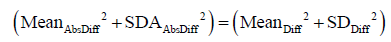
Here we use population definition of SD to calculate  :
:
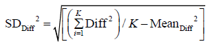
Where Diffi (with i=1…K) stands for individual difference between a pair of measurements performed on the ith of K samples.
Therefore,
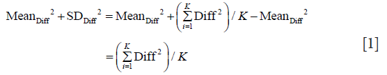
In the same manner we calculate SDAbsDiff and obtain:
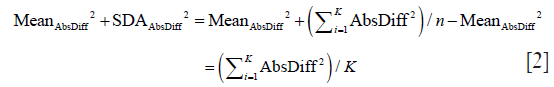
As algebraically, (AbsDiffi)2 = (|Diffi|)2 = (Diffi)2, we prove this identity.
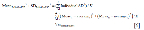
(II) In a next step we prove that (MeanAbsDiff2 + SDAbsDiff2)/2 = MeanIndividual SD2 + SDIndividual SD2
To prove this, it is sufficient to prove that each individual SD calculated from the pair of measurements equals absolute difference of that pair of measurements divided by √2.
Individual SD is calculated by taking the square root of individual variance (Varindividual): Varindividual = [∑(Measurementi-Measurementaverage)2/n−1)]
As only two measurements (Meas1,2) per sample are taken, n−1=1 so the equation for individual variance (Varindividual) becomes:
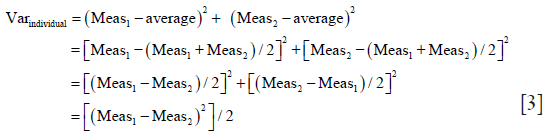
Thus, individual 
With which we prove that for every sample each individual SD calculated from the pair of measurements equals absolute difference of that pair of measurements divided by √2.
(III) Finally we prove that 
As we mention in the text, we use analysis of variance (ANOVA) to calculate observer variance [Varintra(inter)obs] by treating samples as groups, replicate measurements representing within-group variability and within-group mean square (MSwithin) term representing observer variance. MSwithin in one way ANOVA is:

Where Yij is the jth observation in the ith out of K samples and N overall number of measurements, while n represents a number of measurements per sample and K = number of samples. As in this particular case there are 2 measurements per sample therefore n =2 and N = 2K, observer variance (Varintra(inter)obs) becomes
Note that term  is identical to the individual variance (i.e., square of individual SD, equation 4).
We can then generalize Eq. [2] to write
With that we prove the above identity.
Supplementary
The first two columns of Table S1. represent a computer generated simulation mimicking two measurements of LV end diastolic diameter (EDD) obtained by a single observer (Observer One) on 20 subjects averaging 5.0 cm and ranging from 4 to 6 cm, with differences from a true mean having a standard deviation of 0.15 cm and a mean value of 0. The additional columns represent corresponding absolute and relative measures of intraobserver variability calculated from the first two columns. Note that sum of squares of the averages and standard deviations calculated for the absolute difference and difference is equal. Also note that the sum of squares of the average and standard deviation of individual SDs is equal to mean square (MS) error calculated by one-way ANOVA (see Table S2).
Below are two steps of calculating intraclass correlation coefficient (ICC) from the first two columns of Table S1. In a first step ANOVA table is generated (Table S2).
In a second step ICC is calculated as:

Where m equals number of observations (trials); in this case is equal two. In this particular case, intraclass correlation coefficient is very similar to standard correlation coefficient. Also take note that the square root of the error term of this one-way ANOVA is identical to standard error of measurement (SEM) of this particular observer. Finally, please note that intraclass correlation coefficient is equal to 1 minus the ratio between the SEM squared and total (population) variance, in this particular case:
ICC = 1 – 0.142/(12.8/40) =0.94
Again, as the subject variability is a major part of total variability, larger the subject variability, larger the ICC (and vice versa) even if no changes in SEM occur. This lack of relationship is shown in Figure 2. Table S3 shows the original data from Figure 2, along individual SEM intra and ICC.

Calculating SEM
In a next example, inter and intraobserver variability of an experiment involving three observers (each of which measured each sample twice) will be evaluated using standard error of measurement (SEM). Table S4. shows, in addition to measurements made by the Observer One, two additional observers, of which the Observer Two overestimates the true values by 5% while Observer Three underestimates by 4%, with variability around these changed estimates of true value again having a standard deviation of 0.15 cm and mean value of 0. First step of analysis is obtaining a two-factor ANOVA table. But prior to that, we must first restructure the table (Table S5). represents a restructured table.

Full table

Full table
In a step 1 (Table S6) we obtain ANOVA table.

Full table
In step 2, in order to calculate appropriate SEMs we first need to obtain corresponding variances (in Tables S7 and S8 abbreviated by a sign of σ2) using MS of the error (MSE), observer (MSobserver), and observer x subject interaction (MSOxS) components of ANOVA (Table S7). Intraobserver variance (also known as repeatability) is identical to MS error. Observer variance (also known as reproducibility) is calculated from observer and interaction MSs and corresponding degrees of freedom (calculated as nxm). Interaction variance is calculated from observer and error MSs (with m as degrees of freedom); of note, it can be negative, and if so it is neglected. Interobserver variability variance represents the sum of Intraobserver variance, observer variance and interaction variance.

Full table
Finally, corresponding SEMs are calculated by taking a square root of variances (Table S8). Of note, there is a difference between calculations of interobserver variability for fixed or random effects. In usual clinical setting, where the sample of observers that are tested is thought to be randomly selected from a large population of observers, random effects are almost always used. In a particular setting where measurements are always performed by the same group of observers, fixed effects are used.

Full table
Calculating confidence intervals (CIs) for intraobserver SEM
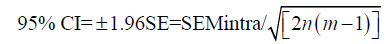
We are assuming that variability of measurements of individual sample follows normal distribution. If we also assume that there is no significant observer impact (which can be tested using ANOVA), then standard error (SE) of intraobserver SEM is:
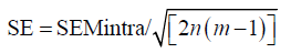
with n(m − 1) being degrees of freedom, where n is number of samples and m is number of observations per sample. If there is a significant impact of observers, the degrees of freedom can be replaced by the degrees of freedom of the error term. 95% CIs are obtained by multiplying standard error by 1.96 for samples with n>30. Otherwise, t test statistics should be used.
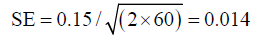
To demonstrate calculation of standard error of SEMintra, let us use our example of 3 observers measuring twice each of the 20 samples (Table S4), and assume that observer impact was not present. Then:
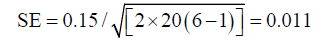
Thus, 95% CIs are 0.129−1.71
As in this particular example there is an observer impact, and therefore 60 degrees of freedom should be used:
With 95% CIs of 0.122−0.177.
Determining sample size
One way to determine sample size is to a priori select the width of the CI for the SEM. Let us assume that we want to have CIs that are within 20% of the value of intraobserver SEM, and that we will use 3 observers that will measure each sample twice. We already know that:
Then, the number of samples measured (n) is:

If we want to double the precision we will need:

In other words, for every doubling of precision, we need four times larger sample.
Comparing two SEMs
Unpaired data can be compared using F-test statistics. For paired data, t test statistics for observer variability can be calculated using the method of Mitchell et al., where:
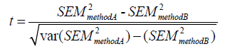
Where var (SEM2) equals:
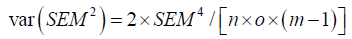
Where n equals number of subjects (samples), o number of observers, and m equals the number of measurements per observer per subject.
Let us assume that in a study that involved 10 subjects, 3 observers and 2 repeated measurements, we compared intraobserver variabilities of 2-dimensional and 3 dimensional ejection fraction measurements, and that we obtained corresponding SEMs of 6% and 4%. The corresponding t test statistics is
With two tailed p value of 0.023.
Acknowledgements
Funding: Funded by the National Space Biomedical Research Institute through NASA cooperative Agreement NCC9-58.
Footnote
Conflicts of Interest: The authors have no conflicts of interest to declare.
References
- Measurement Systems Analysis Workgroup AIAG. Measurement and systems analysis reference manual. Auromotive Industry Action Group; 2010.
- Thavendiranathan P, Popovic ZB, Flamm SD, et al. Improved interobserver variability and accuracy of echocardiographic visual left ventricular ejection fraction assessment through a self-directed learning program using cardiac magnetic resonance images. J Am Soc Echocardiogr 2013;26:1267-73. [Crossref] [PubMed]
- Lim P, Buakhamsri A, Popovic ZB, et al. Longitudinal strain delay index by speckle tracking imaging: A new marker of response to cardiac resynchronization therapy. Circulation 2008;118:1130-7. [Crossref] [PubMed]
- Kusunose K, Penn MS, Zhang Y, et al. How similar are the mice to men? Between-species comparison of left ventricular mechanics using strain imaging. PLoS One 2012;7:e40061. [Crossref] [PubMed]
- Bland JM, Altman DG. Measurement error and correlation coefficients. BMJ 1996;313:41-2. [Crossref] [PubMed]
- Shrout PE, Fleiss JL. Intraclass correlations: Uses in assessing rater reliability. Psychol Bull 1979;86:420-8. [Crossref] [PubMed]
- Bland JM, Altman DG. Statistical methods for assessing agreement between two methods of clinical measurement. Lancet 1986;1:307-10. [Crossref] [PubMed]
- Eliasziw M, Young SL, Woodbury MG, et al. Statistical methodology for the concurrent assessment of interrater and intrarater reliability: Using goniometric measurements as an example. Phys Ther 1994;74:777-88. [Crossref] [PubMed]
- Bland MJ. What is the standard error of the within-subject standard deviation, sw? 2011;2014. Available online: https://www-users.york.ac.uk/~mb55/meas/seofsw.htm
- Greenwod JA, Sandomire MM. Sample size required for estimating the standard deviation as a per cent of its true value. J Am Stat Assoc 1950;45:257-60. [Crossref]
- Bland MJ. How can I decide the sample size for a repeatability study? 2010;2013. Available online: https://www-users.york.ac.uk/~mb55/meas/sizerep.htm
- Thavendiranathan P, Grant AD, Negishi T, et al. Reproducibility of echocardiographic techniques for sequential assessment of left ventricular ejection fraction and volumes: Application to patients undergoing cancer chemotherapy. J Am Coll Cardiol 2013;61:77-84. [Crossref] [PubMed]
- Mitchell JR, Karlik SJ, Lee DH, et al. The variability of manual and computer assisted quantification of multiple sclerosis lesion volumes. Med Phys 1996;23:85-97. [Crossref] [PubMed]

